- Overview
- Configuration
- NTP4 Plug-In
- Hardware
- RFC 868
- RFC 2030
-
RFC 1305
- RFC 1305
- 1. Introduction
- 1.1 Related Technology
- 2. System Architecture
- 2.1 Implementation Model
- 2.2 Network Configurations
- 3. Network Time Protocol
- 3.1 Data Formats
- 3.2 State Variables and Parameters
- 3.2.1 Common Variables
- 3.2.2 System Variables
- 3.2.3 Peer Variables
- 3.2.4 Packet Variables
- 3.2.5 Clock-Filter Variables
- 3.2.6 Authentication Variables
- 3.2.7 Parameters
- 3.3 Modes of Operation
- 3.4 Event Processing
- 3.4.1 Notation Conventions
- 3.4.2 Transmit Procedure
- 3.4.3 Receive Procedure
- 3.4.4 Packet Procedure
- 3.4.5 Clock-Update Procedure
- 3.4.6 Primary-Clock Procedure
- 3.4.7 Initialization Procedures
- 3.4.7.1 Initialization Procedure
- 3.4.7.2 Initialization-Instantiation Procedure
- 3.4.7.3 Receive-Instantiation Procedure
- 3.4.7.4 Primary Clock-Instantiation Procedure
- 3.4.8 Clear Procedure
- 3.4.9 Poll-Update Procedure
- 3.5 Synchronization Distance Procedure
- 3.6 Access Control Issues
- 4. Filtering and Selection Algorithms
- 4.1 Clock-Filter Procedure
- 4.2 Clock-Selection Procedure
- 4.2.1 Intersection Algorithm
- 4.2.2. Clustering Algorithm
- 5. Local Clocks
- 5.1 Fuzzball Implementation
- 5.2 Gradual Phase Adjustments
- 5.3 Step Phase Adjustments
- 5.4 Implementation Issues
- 6. Acknowledgments
- 7. References
- Appendix A
- Appendix B
- Appendix C
- Appendix D
- Appendix E
- Appendix F
- Appendix G
- Appendix H
- Appendix I
- Time Tools
- NTP Auditor
- About
| Previous Top Next |
Windows Time Server
Appendix FThe NTP Clock-Combining Algorithm
Introduction
A common problem in synchronization subnets is systematic time-offset errors resulting from asymmetric transmission paths, where the networks or transmission media in one direction are substantially different from the other. The errors can range from microseconds on high-speed ring networks to large fractions of a second on satellite/landline paths. It has been found experimentally that these errors can be considerably reduced by combining the apparent offsets of a number of time servers to produce a more accurate working offset. Following is a description of the combining method used in the NTP implementation for the Fuzzball [MIL88b]. The method is similar to that used by national standards laboratories to determine a synthetic laboratory time scale from an ensemble of cesium clocks [ALL74b]. These procedures are optional and not required in a conforming NTP implementation.
In the following description the stability of a clock is how well it can maintain a constant frequency, the accuracy is how well its frequency and time compare with national standards and the precision is how precisely these quantities can be maintained within a particular timekeeping system. Unless indicated otherwise, The offset of two clocks is the time difference between them, while the skew is the frequency difference (first derivative of offset with time) between them. Real clocks exhibit some variation in skew (second derivative of offset with time), which is called drift.
Determining Time and Frequency
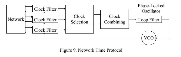
Figure 9 shows the overall organization of the NTP time-server model. Timestamps exchanged with possibly many other subnet peers are used to determine individual roundtrip delays and clock offsets relative to each peer as described in the NTP specification. As shown in the figure, the computed delays and offsets are processed by the clock filter to reduce incidental timing noise and the most accurate and reliable subset determined by the clock-selection algorithm. The resulting offsets of this subset are first combined as described below and then processed by the phase-locked loop (PLL). In the PLL the combined effects of the filtering, selection and combining operations is to produce a phase-correction term. This is processed by the loop filter to control the local clock, which functions as a voltage-controlled oscillator (VCO). The VCO furnishes the timing (phase) reference to produce the timestamps used in all calculations.
Clock Modelling
The International Standard (SI) definition of time interval is in terms of the standard second: the duration of 9,192,631,770 periods of the radiation corresponding to the transition between the two hyperfine levels of the ground state of the cesium-133 atom. Let u represent the standard unit of time interval so defined and v = 1 over u be the standard unit of frequency. The epoch, denoted by t, is defined as the reading of a counter that runs at frequency v and began counting at some agreed initial epoch t0, which defines the standard or absolute time scale. For the purposes of the following analysis, the epoch of the standard time scale, as well as the time indicated by a clock will be considered continuous. In practice, time is determined relative to a clock constructed from an atomic oscillator and system of counter/dividers, which defines a time scale associated with that particular oscillator. Standard time and frequency are then determined from an ensemble of such timescales and algorithms designed to combine them to produce a composite time scale approximating the standard time scale.
Let T(t) be the time displayed by a clock at epoch t relative to the standard time scale:
T(t) = 1/2 D(t sub 0 )[t - t sub 0 ] sup 2 + R(t sub 0 )[t - t sub 0 ] + T(t sub 0 ) + x(t),
where D(t sub 0 ) is the fractional frequency drift per unit time, R(t sub 0 ) the frequency and T(t sub 0 ) the time at some previous epoch t0. In the usual stationary model these quantities can be assumed constant or changing slowly with epoch. The random nature of the clock is characterized by x(t), which represents the random noise (jitter) relative to the standard time scale. In the usual analysis the second-order term D(t sub 0 ) is ignored and the noise term x(t) modelled as a normal distribution with predictable spectral density or autocorrelation function.
The probability density function of time offset p (t - T(t)) usually appears as a bell-shaped curve centered somewhere near zero. The width and general shape of the curve are determined by x(t), which depends on the oscillator precision and jitter characteristics, as well as the measurement system and its transmission paths. Beginning at epoch t0 the offset is set to zero, following which the bell creeps either to the left or right, depending on the value of R(t sub 0 ) and accelerates depending on the value of D(t sub 0 ).
Development of a Composite Timescale
Now consider the time offsets of a number of real clocks connected by real networks. A display of the offsets of all clocks relative to the standard time scale will appear as a system of bell-shaped curves slowly precessing relative to each other, but with some further away from nominal zero than others. The bells will normally be scattered over the offset space, more or less close to each other, with some overlapping and some not. The problem is to estimate the true offset relative to the standard time scale from a system of offsets collected routinely between the clocks.
A composite time scale can be determined from a sequence of offsets measured between the n clocks of an ensemble at nominal intervals tau. Let R sub i (t sub 0 ) be the frequency and T sub i (t sub 0 ) the time of the ith clock at epoch t0 relative to the standard time scale and let "^" designate the associated estimates. Then, an estimator for Ti computed at t0 for epoch t sub 0 + tau is
![]()
neglecting second-order terms. Consider a set of n independent time-offset measurements made between the clocks at epoch t sub 0 + tau and let the offset between clock i and clock j at that epoch be T sub ij (t sub 0 + tau ), defined as
![]()
Note that T sub ij = - T sub ji and T sub ii = 0. Let w sub i ( tau ) be a previously determined weight factor associated with the ith clock for the nominal interval tau. The basis for new estimates at epoch t sub 0 + tau is
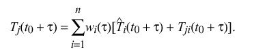
That is, the apparent time indicated by the jth clock is a weighted average of the estimated time of each clock at epoch t sub 0 + tau plus the time offset measured between the jth clock and that clock at epoch t sub 0 + tau.
An intuitive grasp of the behavior of this algorithm can be gained with the aid of a few examples. For instance, if w sub i ( tau ) is unity for the ith clock and zero for all others, the apparent time for each of the other clocks is simply the estimated time T hat sub i (t sub 0 + tau ). If w sub i ( tau ) is zero for the ith clock, that clock can never affect any other clock and its apparent time is determined entirely from the other clocks. If w sub i ( tau ) = 1 / n for all i, the apparent time of the ith clock is equal to the average of the time estimates computed at t0 plus the average of the time offsets measured to all other clocks. Finally, in a system with two clocks and w sub i ( tau ) = 1 / 2 for each, and if the estimated time at epoch t sub 0 + tau is fast by 1 s for one clock and slow by 1 s for the other, the apparent time for both clocks will coincide with the standard time scale.
In order to establish a basis for the next interval tau, it is necessary to update the frequency estimate R hat sub i (t sub 0 + tau ) and weight factor w sub i ( tau ). The average frequency assumed for the ith clock during the previous interval tau is simply the difference between the times at the beginning and end of the interval divided by tau. A good estimator for R sub i (t sub 0 + tau ) has been found to be the exponential average of these differences, which is given by
R hat sub i (t sub 0 + tau ) = R hat sub i (t sub 0 ) + alpha sub i [ R hat sub i (t sub 0 ) - {T sub i (t sub 0 + tau ) - T sub i (t sub 0 )} over tau ],
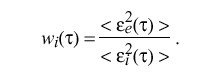
where alpha sub i is an experimentally determined weight factor which depends on the estimated frequency error of the ith clock. In order to calculate the weight factor w sub i ( tau ), it is necessary to determine the expected error epsilon sub i ( tau ) for each clock. In the following, braces "|" indicate absolute value and brackets "<>" indicate the infinite time average. In practice, the infinite averages are computed as exponential time averages. An estimate of the magnitude of the unbiased error of the ith clock accumulated over the nominal interval tau is
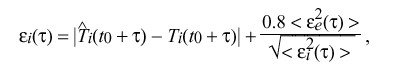
where epsilon sub i ( tau ) and epsilon sub e ( tau ) are the accumulated error of the ith clock and entire clock ensemble, respectively. The accumulated error of the entire ensemble is
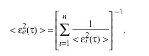
Finally, the weight factor for the ith clock is calculated as
When all estimators and weight factors have been updated, the origin of the estimation interval is shifted and the new value of t0 becomes the old value of t sub 0 + tau.
While not entering into the above calculations, it is useful to estimate the frequency error, since the ensemble clocks can be located some distance from each other and become isolated for some time due to network failures. The frequency-offset error in Ri is equivalent to the fractional frequency yi,
y sub i = { nu sub i~-~nu sub I } over nu sub I
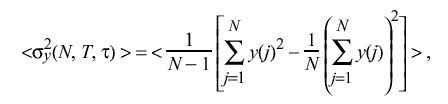
measured between the ith time scale and the standard time scale I. Temporarily dropping the subscript i for clarity, consider a sequence of N independent frequency-offset samples y(j) (j= 1, 2,... ,N) where the interval between samples is uniform and equal to T. Let tau be the nominal interval over which these samples are averaged. The Allan variance sigma sub y sup 2 ( N,T,tau ) [ALL74a] is defined as
A particularly useful formulation is N = 2 and T = tau:
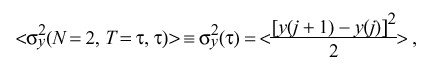
so that
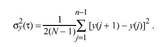
While the Allan variance has found application when estimating errors in ensembles of cesium clocks, its application to NTP is limited due to the computation and storage burden. As described in the next section, it is possible to estimate errors with some degree of confidence using normal byproducts of NTP processing algorithms.
Application to NTP
The NTP clock model is somewhat less complex than the general model described above. For instance, at the present level of development it is not necessary to separately estimate the time and frequency of all peer clocks, only the time and frequency of the local clock. If the timekeeping reference is the local clock itself, then the offsets available in the peer.offset peer variables can be used directly for the T sub ij quantities above. In addition, the NTP local-clock model incorporates a type-II phase-locked loop, which itself reliably estimates frequency errors and corrects accordingly. Thus, the requirement for estimating frequency is entirely eliminated.
There remains the problem of how to determine a robust and easily computable error estimate epsilon sub i. The method described above, although analytically justified, is most difficult to implement. Happily, as a byproduct of the NTP clock-filter algorithm, a useful error estimate is available in the form of the dispersion. As described in the NTP specification, the dispersion includes the absolute value of the weighted average of the offsets between the chosen offset sample and the n-1 other samples retained for selection. The effectiveness of this estimator was compared with the above estimator by simulation using observed timekeeping data and found to give quite acceptable results.
The NTP clock-combining algorithm can be implemented with only minor modifications to the algorithms as described in the NTP specification. Although elsewhere in the NTP specification the use of general-purpose multiply/divide routines has been successfully avoided, there seems to be no way to avoid them in the clock-combining algorithm. However, for best performance the local-clock algorithm described elsewhere in this document should be implemented as well, since the combining algorithms result in a modest increase in phase noise which the revised local-clock algorithm is designed to suppress.
Clock-Combining Procedure
The result of the NTP clock-selection procedure is a set of survivors (there must be at least one) that represent truechimers, or correct clocks. When clock combining is not implemented, one of these peers, chosen as the most likely candidate, becomes the synchronization source and its computed offset becomes the final clock correction. Subsequently, the system variables are adjusted as described in the NTP clock-update procedure. When clock combining is implemented, these actions are unchanged, except that the final clock correction is computed by the clock-combining procedure.
The clock-combining procedure is called from the clock-select procedure. It constructs from the variables of all surviving peers the final clock correction THETA. The estimated error required by the algorithms previously described is based on the synchronization distance LAMBDA computed by the distance procedure, as defined in the NTP specification. The reciprocal of LAMBDA is the weight of each clock-offset contribution to the final clock correction. The following pseudo-code describes the procedure.
begin clock-combining procedure
temp1 <-- 0;
temp2 <-- 0;
for (each peer remaining on the candidate list) /* scan all survivors */
LAMBDA <-- distance (peer);
temp <-- 1 over peer.stratum * NTP.MAXDISPERSE + LAMBDA;
temp1 <-- temp1 + temp; /* update weight and offset */
temp2 <-- temp2 + temp * peer.offset;
endif;
THETA <-- temp2 over temp1;
/* compute final correction */
end clock-combining procedure;
The value THETA is the final clock correction used by the local-clock procedure to adjust the clock.